Bayes Classification

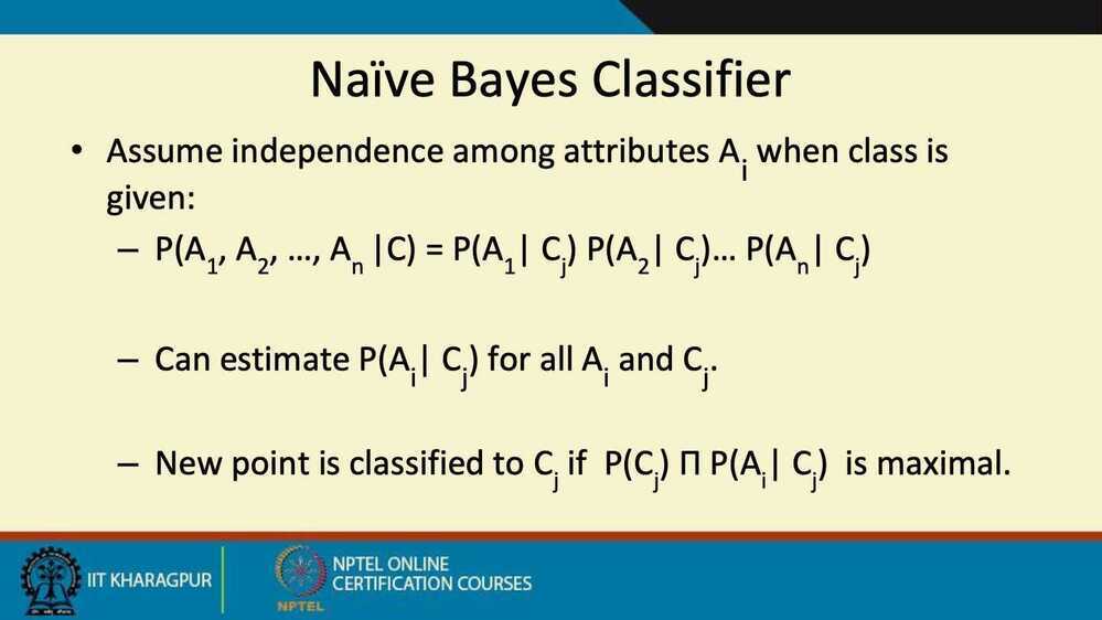
Naive Bayes

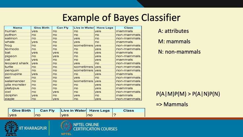
Naive Bayes is a simple but surprisingly powerful algorithm for predictive modeling.

The model is comprised of two types of probabilities that can be calculated directly from your training data:

1. The probability of each class.
2. The conditional probability for each class given each x value.

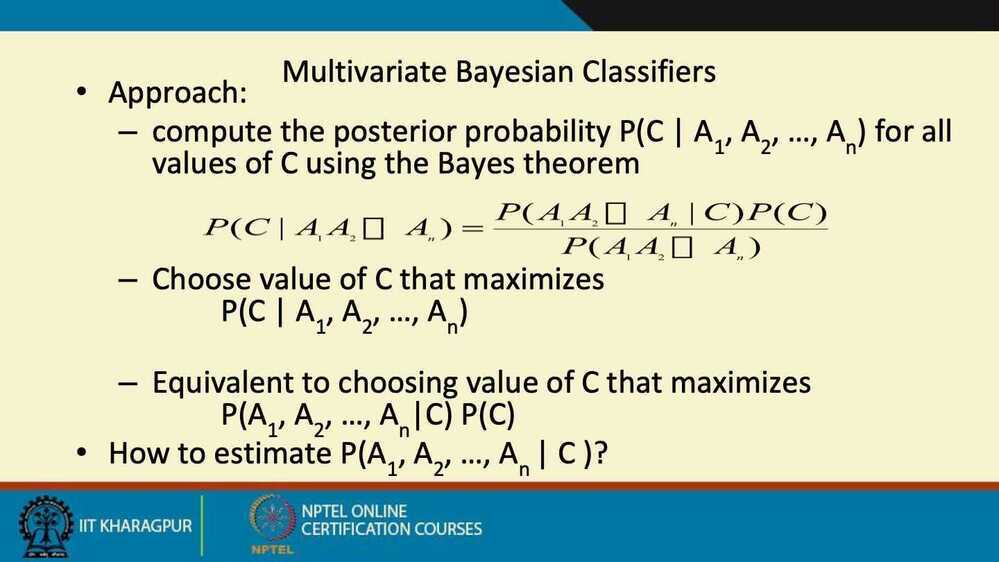
Once calculated, the probability model can be used to make predictions for new data using Bayes Theorem.

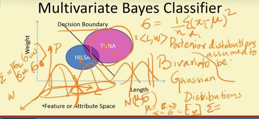
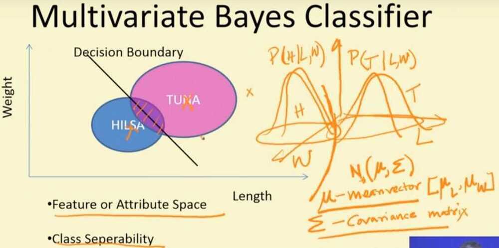
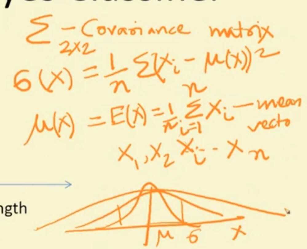
When your data is real-valued it is common to assume a Gaussian distribution (bell curve) so that you can easily estimate these probabilities.

Naive Bayes is called naive because it assumes that each input variable is independent. This is a strong assumption and unrealistic for real data, nevertheless, the technique is very effective on a large range of complex problems.

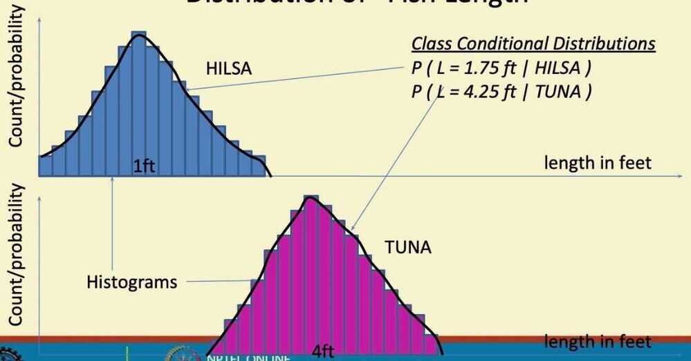
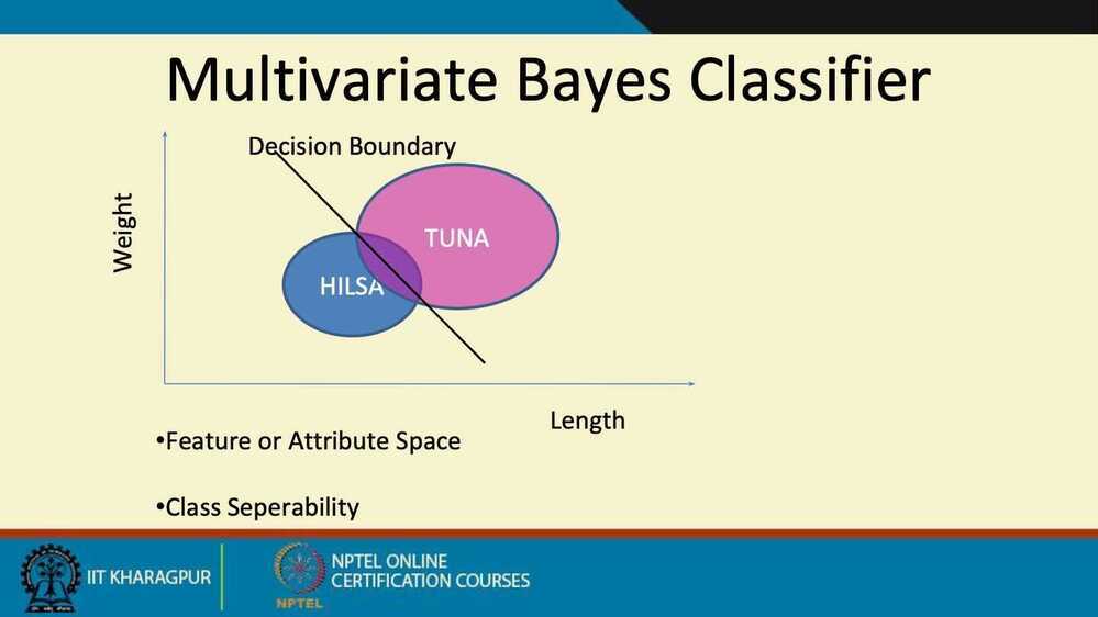
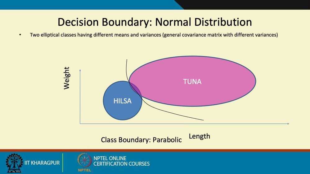
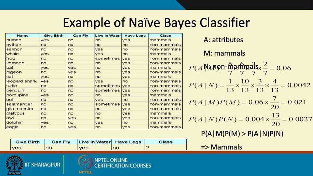
A simple species classification problem

• Measure the length of a fish, and decide its class - Hilsa or Tuna
• Collect Statistics
• Distribution of "Fish Length"

• Decision Rule
  • If length L <= B
    • Hilsa
  • Else
    • Tuna
  • What should be the value of B ("boundary" length)
    • Based on population statistics
• Error of Decision Rule

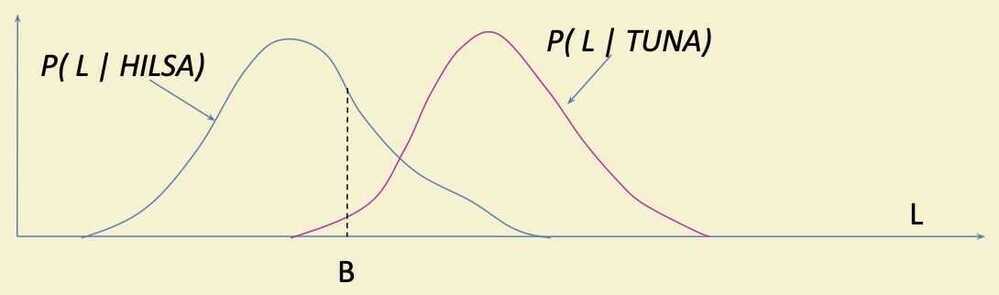
Errors: Type 1 + Type 2

Type 1: Actually Tuna, Classified as Hilsa (area under pink curve to the left of a B)

Type 2: Actually Hilsa, Classified as Tuna (area under blue curve to the right of a B)

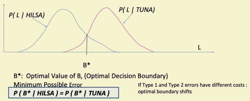
• Optimal Decision Rule

• Species Identification Problem

  • Measure lengths of a (sizeable) population of Hilsa and Tuna fishes
  • Estimate Class Conditional Distributions for Hilsa and Tuna classes respectively
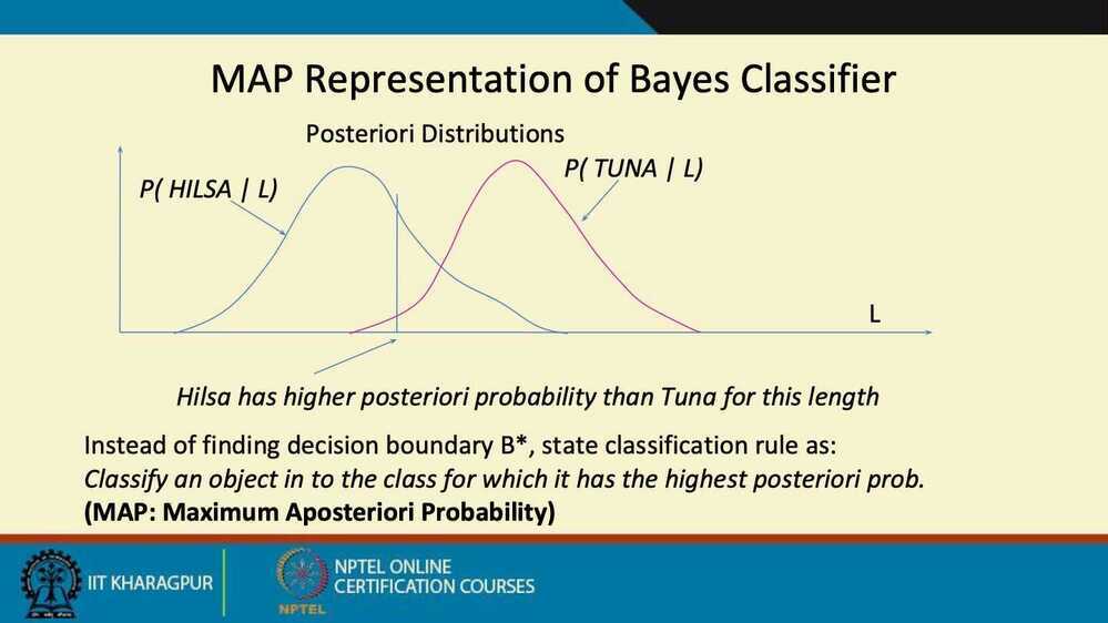
  • Find Optimal Decision Boundary B* from the distributions
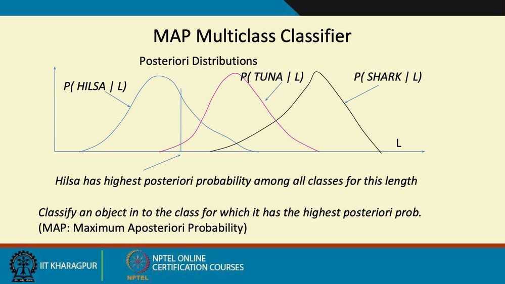
  • Apply Decision Rule to classify a newly caught (and measured) fish as either Hilsa or Tuna
    • with minimum error probability

• Location / Time of Experiment

  • Calcutta in Monsoon
    • More Hilsa few Tuna
  • California in Winter
    • More Tuna less Hilsa
  • Even a 2ft fish is likely to be Hilsa in Calcutta a 1.5ft fish may be Tuna in California

• If the distribution is biased, we can scale up the class conditional probability to make b* optimal.

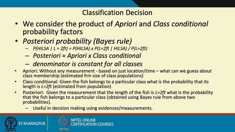
• We can do the scaling using Apriori Probability

Apriori Probability

• Without measuring lengh what can we guess about the class of a fish

  • Depends on location / time of experiment
    • Calcutta: Hilsa, California: Tuna

• Apriori probability: P(HILSA), P(TUNA)

  • Property of the frequency of classes during experiment
    • Not a property of length of the fish
  • Calcutta: P(Hilsa) = 0.90, P(Tuna) = 0.10
  • California: P(Tuna) = 0.95, P(Hilsa) = 0.05
  • London: P(Tuna) = 0.50, P(Hilsa) = 0.50

• Also a determining factor in class decision along with class conditional probability

• We multiply the class conditional curve by the Apriori Probability

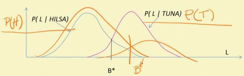
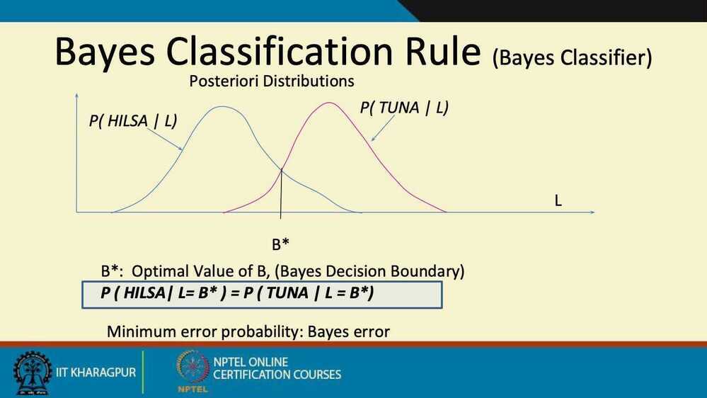
• Also called Bayes Optimal Classifier
• and B* is called Bayes Optimal Boundary

Summary

• Advantages
  • Robust to isolated noise points
  • Handle missing values by ignoring the instance during probability estimate calculations
  • Robus to irrelevant attributes
• Drawback
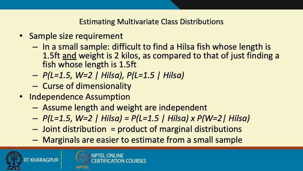
  • Independence assumption may not hold for some attributes
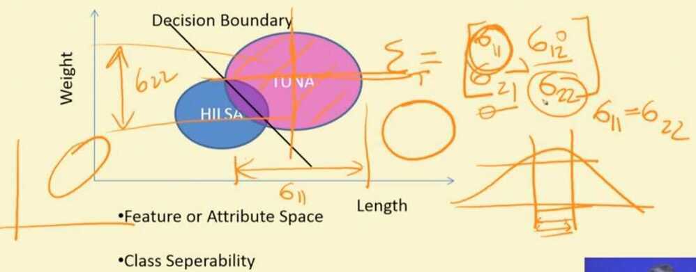
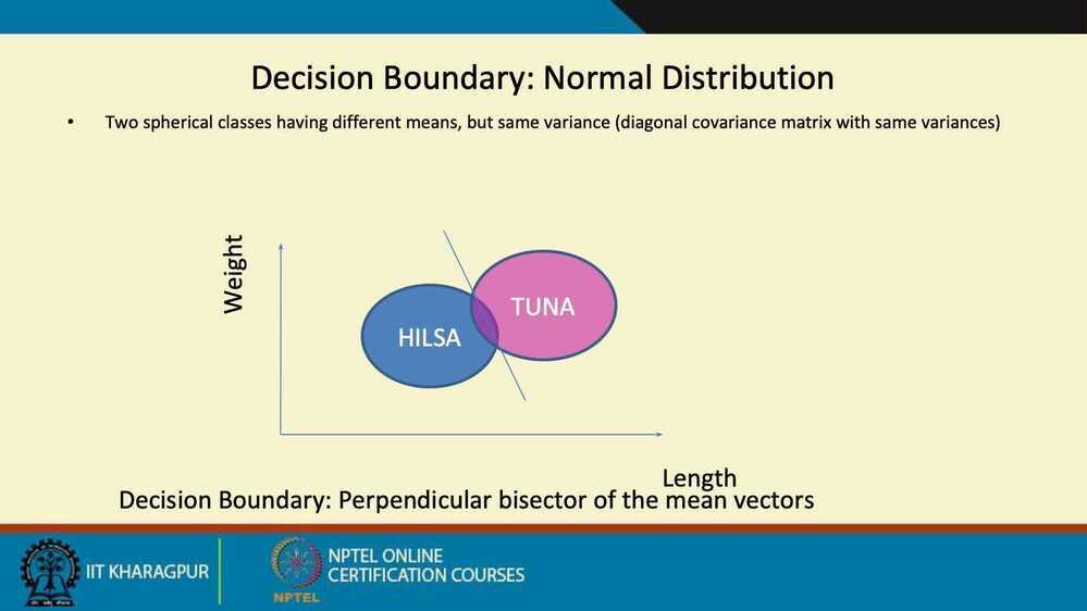
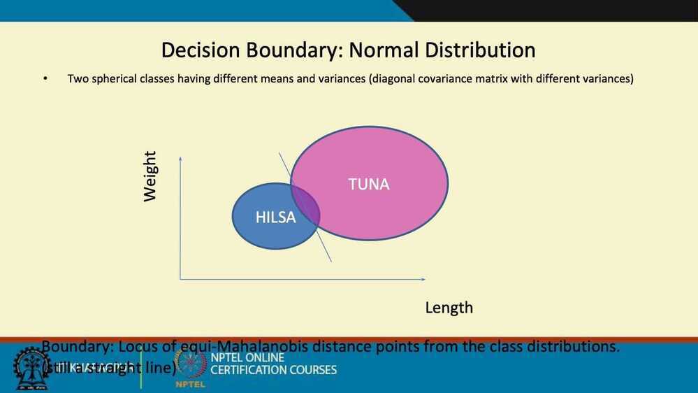
    • Lenght and weight of a fish are not independent
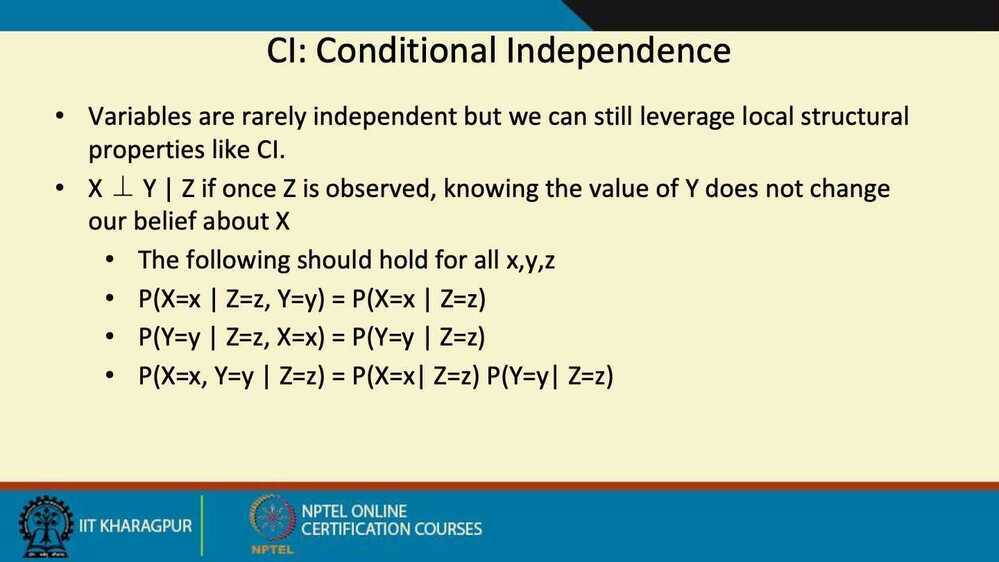
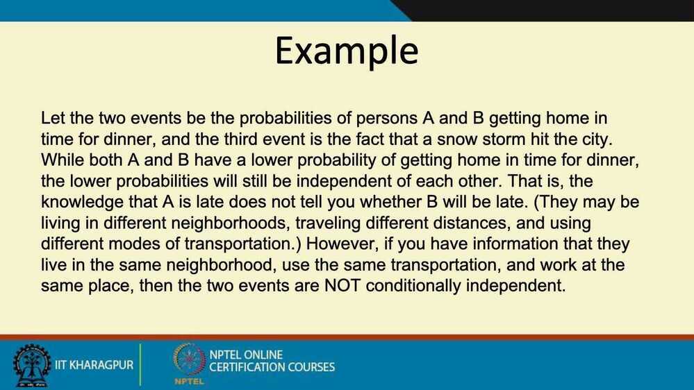
    • Conditional Independence