Word Embedding to Transformers

1. Introduction

Natural language processing (NLP) is an active research field of linguistic, computer science and artificial intelligence. The main goal of NLP is the capability of a computer to understand content in texts or documents. There are many different challenging tasks to solve in the field of NLP:

• Machine Translation: is the task of translating a sentence x from one language to a sentence y in another language. Therefore one of the most popular example is: www.deepl.com
• Text classification: Text classification is the process of understanding the meaning of unstructured text and organizing it into predefined categories (tags). One of the most popular text classification task is sentiment analysis, which aims to categorize unstructured data by sentiments. A basic task in text classification / sentiment analysis is classifying the polarity of a given text at the document, sentence, or feature/aspect level-whether the expressed opinion in a document, a sentence or an entity feature/aspect is positive, negative, or neutral.
• Semantic analysis: Semantic tasks analyze the structure of sentences, word interactions, and related concepts, in an attempt to discover the meaning of words, as well as understand the topic of a text.
• Part-of-speech tagging: Part-of-speech (PoS) tagging is a popular natural language processing process which refers to categorizing words in a text (corpus) in correspondence with a particular part of speech, depending on the definition of the word and its context. PoS tagging is useful for identifying relationships between words and, therefore, understand the meaning of sentences.
• Text summarization: Text summarization in NLP is the process of summarizing the most important informations in large texts for quicker consumption.
• Generative models for NLP: Generative models are normally trained on a large amount of data, with the ability to create afterwards new texts.

2. NLTK - natural language toolkit

NLTK is a leading platform for building Python programs to work with human language data. It provides easy-to-use interfaces to over 50 corpora and lexical resources such as WordNet, along with a suite of text processing libraries for classification, tokenization, stemming, tagging, parsing, and semantic reasoning, wrappers for industrial-strength NLP libraries, and an active discussion forum.

2.1 Tokenizing

A tokenizer breaks unstructured data and natural language text into chunks of information that can be considered as discrete elements. Normally, it is the first step in each NLP project. The two most common versions of tokenizers are the "word based tokenizing" and the "sentence based tokenizing".

Tokenizing by words

Words are like the atoms of natural language. They are the smallest unit of meaning that still makes sense on its own. Tokenizing a text by word allows to identify words that come up particularly often. For example, if you were analyzing a group of job postings, then you might find that the word "Python" comes up often. That could suggest high demand for Python knowledge, but you would need to look deeper to know more.

Tokenizing by sentence

When you tokenize by sentence, you can analyze how those words relate to one another and see more context.

2.2 Stemming

Stemming and Lemmatization are text normalization (or sometimes called word normalization) techniques in the field of natural language processing that are used to prepare text, words, and documents for further processing, because the mathematical models needs a vector description of a word or a sentence, and can not work with "strings" directly. Stemming and Lemmatization have been studied, and algorithms have been developed in Computer Science since the 1960’s.

Stemming is a text processing task in which reduces words to their root, which is the core part of a word. For example, the words "helping" and "helper" share the root "help". Stemming allows to zero in on the basic meaning of a word rather than all the details of how it is being used. Stemming a word or sentence may result in words that are not actual words. Stems are created by removing the suffixes or prefixes used with a word. The natural language toolkit (NLTK) contains more than only one stemming algorithm. For the English language, you can choose between PorterStammer or LancasterStammer, PorterStemmer being the oldest one originally developed in 1979. LancasterStemmer was developed in 1990 and uses a more aggressive approach than Porter Stemming Algorithm.

Porter Stemmer

Porter Stemmer uses suffix stripping to produce stems. Notice how the Porter Stemmer is giving mthe root (stem) of the word "cats" by simply removing the "s" after cat. This is a suffix added to cat to make it plural. But if you look at "trouble", "troubling" and "troubled" they are stemmed to "trouble" because Porter Stemmer algorithm does not follow linguistics rather a set of rules for different cases that are applied in phases (step by step) to generate stems. This is the reason why Porter Stemmer does not often generate stems that are actual English words.

Lancaster Stemmer

The Lancaster Stemmer (Paice-Husk stemmer) is an iterative algorithm with rules saved externally. One table containing about 120 rules indexed by the last letter of a suffix. At each iteration, it tries to find an applicable rule by the last character of the word. Each rule specifies either a deletion or replacement of an ending. If there is no such rule, it terminates. It also terminates if a word starts with a vowel and there are only two letters left or if a word starts with a consonant and there are only three characters left. Otherwise, the rule is applied, and the process repeats.

Snowball Stemmer

The Snowball Stemmer is a non-English stemmer. With the Snowball Stemmer it is possible to create a own language stemmer.

2.3 Lemmatizing

Lemmatization, unlike Stemming, reduces the inflected words properly ensuring that the root word belongs to the language. In Lemmatization root word is called Lemma. A lemma (plural lemmas or lemmata) is the canonical form, dictionary form, or citation form of a set of words. For example, runs, running, ran are all forms of the word run, therefore run is the lemma of all these words. Because lemmatization returns an actual word of the language, it is used where it is necessary to get valid words. The Python NLTK library provide the WordNet Lemmatizer that uses the WordNet Database to lookup lemmas of the words.

Now the question may arise, when do I use which method (Stemming or Lemmatizing)?

The Stemmer method is much faster than Lemmatizing, but it produces in general worse results. Using Stemming might end up that the generated stem is not an actual word, because it uses no corpus. It depends a bit on the current problem which you are working on. If you are building a language application in which language and a grammatic is important, then the lemmatizing approach will be better than the stemming approach.

3. Word embeddings

3.1 Overview of word embeddings

In NLP, word embedding is a projection of a word, consisting of characters into meaningful vectors of real numbers. Conceptually it involves a mathematical embedding from a dimension N (all words in a given corpus)-often a simple one-hot encoding is used- to a continuous vector space with a much lower dimensionality, typically 128 or 256 dimensions are used. Word embedding is a crucial preprocessing step for training a neural network. There extists many different approaches for word embedding, which will be explained in the following sections of this blog.

There are two main properties for a useful projection:

• Distributed representation of concepts and continuity of words sharing similar properties
• Allow to learn this projection for the given task

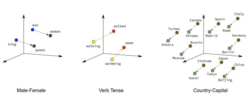
Fig.1 - Illustration of a word embedding

3.2 One-hot encoding

One-hot encoded words are not useful to solve a NLP task successfully. Assume that an arbitrary dictionary consists out of 5000 different words. This means, when using one-hot encoding, each word will be represented by a vector of length 5000, but 4999 of these entries are zero. It can be concluded, that the dimensionality gets very high and the featurespace is very sparse. Additionally there is not any connection of words with a similar meaning, as visible in figure 1 above.

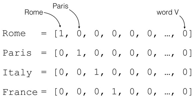
Fig.2 - Example of a one-hot encoding for words

3.3 Embedding layer

A standard approach is, to feed the one-hot encoded tokens (mostly words, or sentence) into a embedding layer. During training the model tries to find a suitable embedding (lower dimensionality as the input layer). The position of a word within the vector space is learned from text and is based on the words that surround the word when it is used. In some cases it could be useful to use a pretrained embedding, which was trained on a hugh corpus of words. Figure 3 shows a schematic architecture of a word based embedding layer.

• Input: one-hot encoding of the word in a vocabulary
• Output: one vector of N dimensions (given by the user, probably tuned with hyperparameter tuning)

There exists many different approaches of word embedding, some of the most popular ones we will look in more detail during the following sections.

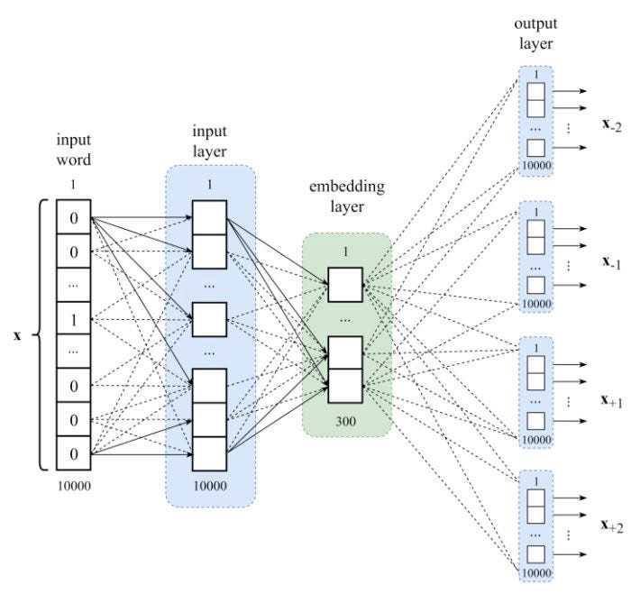
Fig.3 - Visualization of a embedding layer

3.3.1 Training of an embedding layer

There exists three main options to train a embedding layer, and it depends on the natural language processing problem which approach should be chosen, to solve the problem.

Three main options for training a embedding layer:

• Train the weights of the embedding layer from scratch for a given task.
• Use a pretrained embedding such as word2vec, GloVe, FastText, ELMo, (these approaches will be explained in more detail later on).
• Similar approach as for transfer learning: take a pretrained embedding and fine tune it through training (with a very small learningrate, e.g: 1e-5) for the given task.

3.3.2 Keras embedding layer

Keras offers an embedding layer that can be used for neural networks, such as RNN’s (recurrent neural networks) for text data. This layer is defined as the first layer of a more complex architecture. The embedding layer needs at least three input values:

• input_dim: Integer. Size of the vocabulary, i.e. maximum integer index+1.
• output_dim: Integer. Dimension of the dense embedding.
• input_length: Length of input sequences, when it is constant. This argument is required if you are going to connect Flatten then Dense layers upstream (without it, the shape of the dense outputs cannot be computed).

Example:

• e = Embedding(200, 32, input_length=50) → vocabulary with 200 words, output dimension should be 50 and each document will have 50 words

Example of a keras embedding layer

# define the model

model = tf.keras.Sequential()

#vocabulary size = 30, inputlegth = 4, output size = 8

model.add(tf.keras.layers.Embedding(vocabsize, 8, inputlength=maxlength))model.add(tf.keras.layers.Flatten())

#binary classification problem

model.add(tf.keras.layers.Dense(1, activation='sigmoid'))# compile the model

model.compile(optimizer='adam',

loss='binarycrossentropy',

metrics=['accuracy'])# summarize the model

print(model.summary())

Model summary

Model: "sequential_2"

Layer (type) - Output Shape - Param
===
embedding_1 (Embedding) - (None, 4, 8) - 400
flatten_1 (Flatten) - (None, 32) - 0
dense_1 (Dense) - (None, 1) - 33
====
Total params: 433
Trainable params: 433
Non-trainable params: 0
---
None

Results

# fit the model
model.fit(padded_docs, labels, epochs=50, verbose=0)

# evaluate the model
loss, accuracy = model.evaluate(padded_docs, labels, verbose=0)

print('Accuracy: %f' % (accuracy*100))

#100.00

3.4 Word2Vec

Word2Vec relates to a type of models, producing word embedding into space with contextual similarity, i.e. words that share common contexts are located in close proximity. We will explain the three main architectures of the word2Vec approach in the next sections. For more details we refer to the original papers.

One hypothesis of the word2vec approach is, that a word is represented by its "context", or in other words, a window around the target word is created and words falling in the window are added to the "bag" disregarding the order. The word2vec mapping is not only about clustering related words, it is also able to preserve some "path meaning".

For the word2vec approach, there exist many different architecture approaches:

• One word context: uses only one single word as context (this strategy is not often used, mainly a educational approach).
• Skip-gram model: An extension of one word context to multi word context at the output.
• Continuous bag-of-word model: An extension of one word context to multi word context at the input.

3.4.1 One word context model

The one word approach takes only one word as input and tries, based on this input to predtict the output word. This approach is not used widely in practise, it is more an educational approach, because the model can not learn any context in a given document.

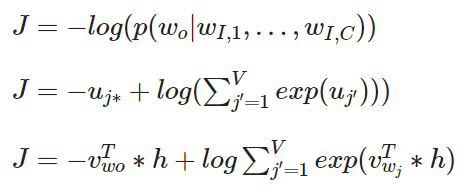
Lossfunction of the one word context model

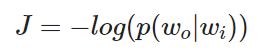
The model simply tries to maximise the negative log of the probability of the output word given the input word.

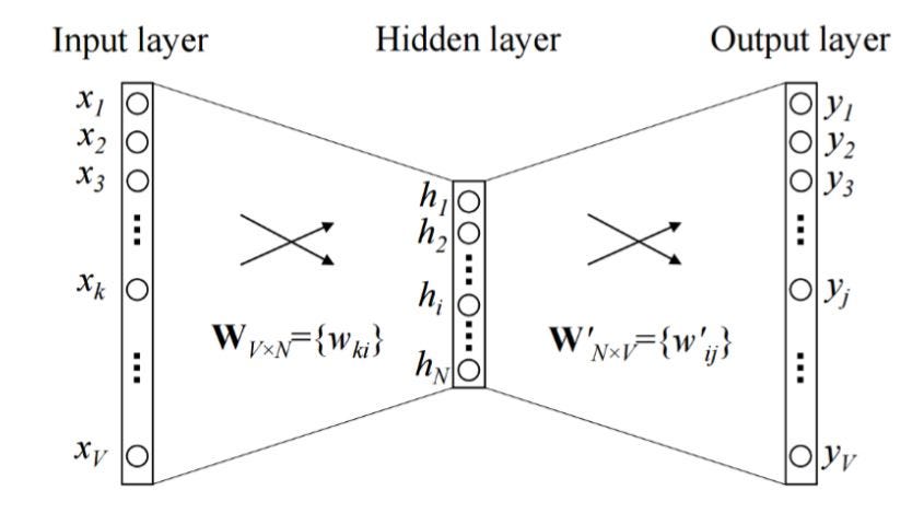
Fig.4 - one word context model

3.4.2 Skip-gram model

A more suitable approach than the one word context model is the skip-gram model. This model takes one target word as input to predict the context (neighbouring words).

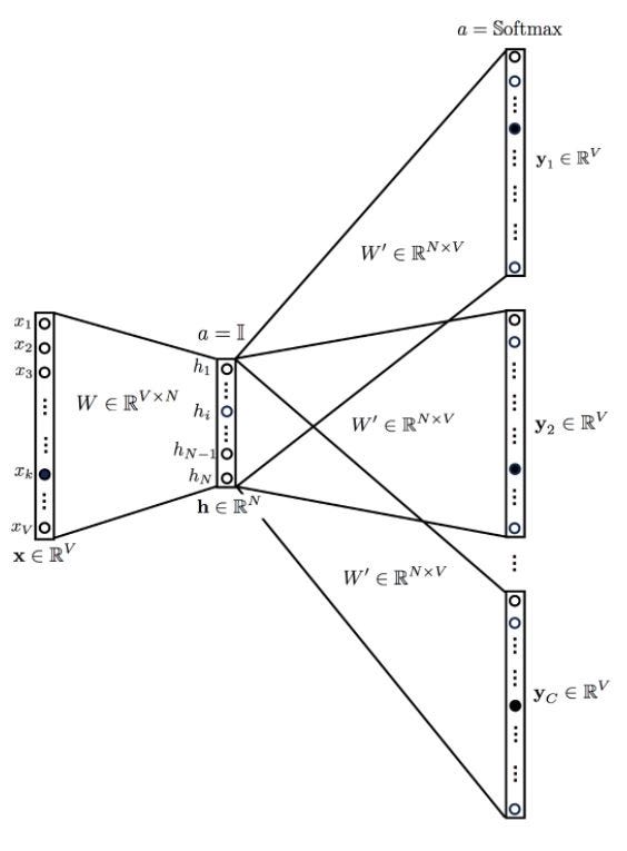
Fig.5 - skip-gram model

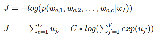
Lossfunction of the skip-gram model

The lossfunction is not very different than the lossfunction of the word context model.

3.4.3 Continuous bag-of-word

In the continuous bag-of-word approach (CBOW) the model tries to predict the actual word based from some surrounding words, in this sense it is the reversed approach of the skip gram model. The order of the surrounding words does not influence the prediction (therefore: bag-of-words).

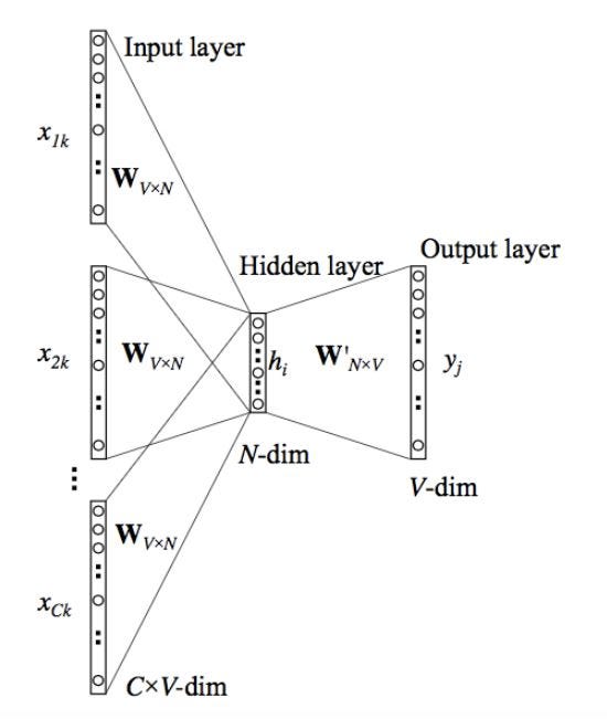
Fig.6 - Continuous bag-of-word model

Lossfunction of the continuous bag-of-word model

The lossfunction is similar to the lossfunction of the one word model. The only difference is that more than one words are given.

More about the mathematical concept behind the model can be found in original paper.

3.5 GloVe - Global vectors for word representation

Another, more advanced approach for word embedding is the GloVe model. GloVe means global vectors for word representation. This approach is not based on a pure ANN (artificial neural network) approach, but also on statistical approaches. The GloVe-approach combines basically the advantages of the word2vec approach and the LSA approach. LSA mean Latent Semantic Analysis and was one of the first approaches for vector embedding of words.

GloVe is an unsupervised learning algorithm for obtaining vector representations for words. Training is performed on aggregated global word-word co-occurrence statistics from a corpus, and the resulting representations showcase interesting linear substructures of the word vector space.

3.5.1 Basic principle of GloVe

Some basic notation first:

• X : is the matrix of word-word co-occurrence. The matrix is quadratic and has the shape of the number of words in the corpus.
• X_i=∑(X_ik) : The number of times any word appears in the context of word i.
• P_ij=P(i|j)=X_ij/X_i : the probability that word j appear in the context of word i.

Given a corpus having V words, the co-occurence matrix X will have the shape of V*V where the i-th row and j-th column of X,X_ij denotes, how many times word i has co-occurred with word j.

As an easy example, we are using the following sentence:

"the cat sat on the mat".

We use a windowsize of "one" for this example, but it is also possible / useful to use a larger window size. Figure 7, shows the resulting co-occurrence matrix of the example sentence above:

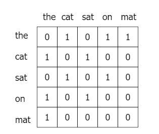
Fig.7 - Example of a simple Co-occurence matrix

To measure the similarity between words, we need three words at a time. The following table shows such an example:

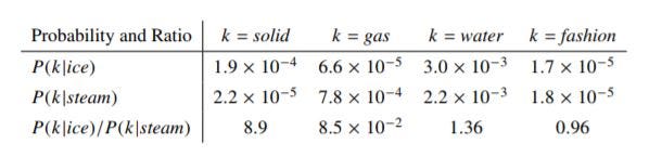
Fig.8 - GloVe probability table

The table above shows the co-occurrence probabilities for target words ice and steam with selected context words from a six billion token corpus. Only in the ratio does noise from non-discriminative words like water and fashion cancel out, so that large values (much greater than one) correlate well with properties specific to ice, and small values (much less than one) correlate well with properties specific of steam.

You can see that given two words, i.e. ice and steam, if the third word k (also called the "probe word"):

• is very similar to ice but irrelevant to steam (e.g. k=solid), P_ik/P_jk will be very high (>1),
• is very similar to steam but irrelevant to ice (e.g. k=gas), P_ik/P_jk will be very small (<1),
• is related or unrelated to either words, then P_ik/P_jk will be close to 1

So, if we can find a way to incorporate P_ik/P_jk to computing word vectors we will be achieving the goal of using global statistics when learning word vectors.

3.5.2 Mathematical background of the GloVe approach

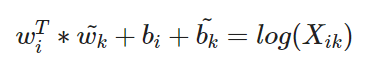
It can be shown, that an appropriate starting point for word vector learning could be working with ratios of co-occurrence probabilities rather then the probabilities themselves. We take the following equation as a starting point:

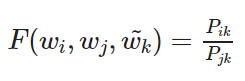
In the formula from above, F() can be taken to be a complicated function parameterized by a neural network. The ratio P_ik/P_jk depends on three words i,j and k. In the formula above are w the word vectors and w_tilde are the separate context vectors.

After some recalculation steps we get to following formula:

A main drawback to this model is that it weights all co-occurrences evenly, even those that happen rarely or never. Such rare co-occurrences are noisy and carry less information than the more frequent ones - yet even just the zero entries account for 75-95% of the data in X, depending on the vocabulary size and corpus. The authors from the GloVe-paper proposed a new weighted least squares regression model that addresses these problems. The weight function f(Xij) is shown in figure 9.

Lossfunction of the GloVe model

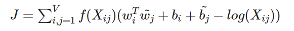
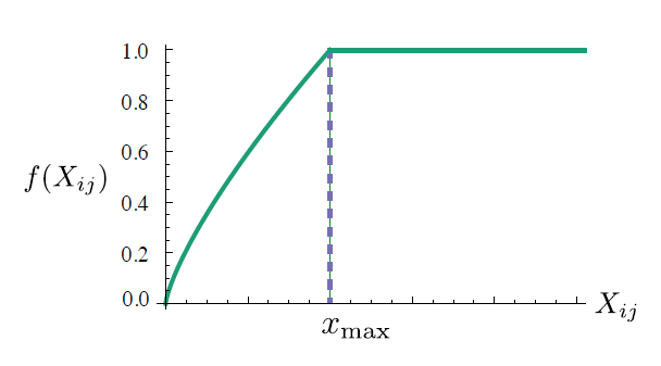
Fig.9 - Example of the weightfunction f(Xij)

3.5.3 Training details of GloVe

Glove is based on matrix factorization techniques on the word-context matrix, also known as the co-occurrence matrix. It first constructs a large matrix of (words - context) co-occurrence information (the violett matrix in figure 10 below), i.e. for each "word" (the rows), we count how frequently we see this word in some "context" (the columns) in a large corpus. The number of "contexts" is of course large, since it is essentially combinatorial in size. The idea then is to apply matrix factorization to approximate this matrix as depicted in the following figure 10.

So then we factorize this matrix to yield a lower-dimensional (word - features) matrix (the orange matrix in figure 10 below), where now each row yields a vector representation for the corresponding word. In general, this is done by minimizing a "reconstruction loss". This loss tries to find the lower-dimensional representations which can explain most of the variance in the high-dimensional data.

Mostly the word-feature matrix and the feature-context matrix are initialized randomly and attempt to multiply them to get a word-context co-occurrence matrix, which is as similar as possible to the original matrix. After training, the word-featrue matrix gives the learned word embedding for each word where the number of columns (features) can be present to a specific number of dimension, given by the user as a hyperparameter.

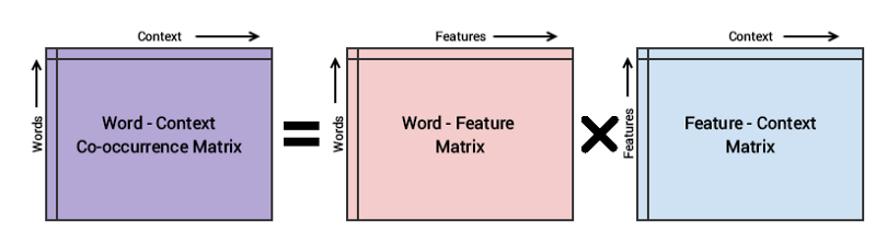
Fig.10 - Conceptual model for the GloVe model

3.6 FastText (enriching word vectors with subword information)

FastText is a extension of the traditional Word2Vec approach, especially the continuous skip-gram model and it was proposed by Facebook. Instead of feeding different individual words into the neural network, FastText breaks down the words into several n-grams, or sub-words. The word embedding vector for a word will be the sum of all of its n-grams.

FastText has one main advantage in contrast to the previous explained methods. This approach can not only represent the words in the vocabulary, but also out-of-vocabulary words can be represented since their n-grams probably appears in other words of the trainingset. This can be very useful for compound words.

3.6.1 Keypoints of FastText

hierarchical softmax

A softmax function is very common used as an activation function to output the probability of a given input to belong to n different classes in multi-class classification problems. Hierarchical softmax proves to be very efficient when there are a large number of categories and there is a class imbalance present in the data. Here, the classes are arranged in a tree distribution instead of a flat, list-like structure. The construction of the hierarchical softmax layer is based on the Huffman coding tree, which uses shorter trees to represent more frequently occurring classes and longer trees for rarer, more infrequent classes. The probability that a given text belongs to a class is explored via a depth-first search along the nodes across the different branches. Therefore, branches (or equivalently, classes) with low probabilities can be discarded away. For data where there are a huge number of classes, this will result in a highly reduced order of complexity, thereby speeding up the classification process significantly compared to traditional models.

A more detailed explanation, also with the mathematics behind can be found in this post.

Word n-grams

Using only a bag of words representation of the text leaves out crucial sequential information. Taking word order into account will end up being computationally expensive for large datasets. So as a happy medium, FastText incorporates a bag of n-grams representation along with word vectors to preserve some informations about the surrounding words appearing near each word. This representation is very useful for classification applications, as the contextual meaning of a couple of different words strung together also results in a particular sentiment echoed by that piece of text.

n-gram hashing

Working with n-grams lead to a very huge number of different n-grams. The FastText approach uses a hashing function to convert each character n-gram to a hashed integer value between 1 and B. This method can dramatically decrease the the size of the bucket.

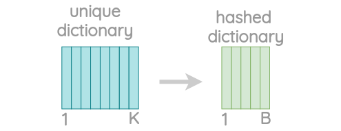
Fig.11 - Visualization of the dictionary reduction

Fig.12 - Visualization of hashing process

3.6.2 Mathematical background of the FastText approach

log-likelihood of the skipgram model (given is the target word, and the model is trained to predict well words that appear in its context):

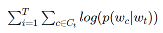
The context C_t is the set of indices of words surrounding word w_t. The skipgram model uses a scoring function, and calcualte the probability p(wc|wt) with a softmax function. The FastText model uses a very similar scoring function but in a slightly different way. In the FastText approach, each word ww will be represented as a bag of n-grams.

Here a simple example:

input word: where → split in n-grams (where n=3): wh, whe, her, ere, re

The main difference between skipgram and FastText is only that the scoring function is the sum over all n-gram vectors.

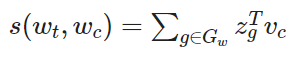
A word will be represented by the sum of the vector representation of its different n-grams. This scoring function is then used for the softmax function, same as in the skipgram approach.

3.6.3 Architecture of FastText

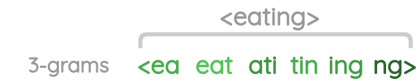
Fig.13 - Architecture overview of the FastText model

3.7 ELMo

All previous presented word embedding approaches have one thing together. They all have exactly one embedding for one word or a n-gram of a word. They do not look at the contextual relationship of a specific word, or only in a very small range and in a limited way (skip gram model).

These approaches have two main problems:

• Always the same representation for a word type, regardless of the context in which a word token occurs.
• We just have one representation for a word, but words have different aspects, including semantics, syntatic behaviour, and register/connotations

In contrast to Word2Vec, ELMo (Embeddings from language models) looks at the entire sentence before assigning each word in its embedding. The ELMo approach makes the step over from simple word embedding, like the approaches shown before to language model.

Here one example where ELMo can help for creating a better embedding:

• "The plane took of at exactly nine o’clock"
• "The plane surface is a must for any cricket pitch"
• "Plane geometry is fun to study"

The word "plane" has in each of this three sentences a completely different meaning.

3.7.1 Keypoints of ELMo

Unlike most widely used word embeddings, ELMo word representations are functions of the entire input sentence. Instead of using a fixed embedding for each word, ELMo looks at the entire sentence before assigning each word in it an embedding. It uses a two layer bi-directional LSTM, trained on a specific task to be able to create those embeddings. As for other word embeddings, it is also possible to use a pretrained version of a ELMo model.

ELMo gained its language understanding from being trained to predict the next word in a sequence of words - a task called Language Modeling. This is convenient because we have vast amounts of text data that such a model can learn from without needing labels.

3.7.2 ELMo architecture

ELMo basically consists out of two bi-directional LSTM layers - so that the language model does not only have a sense of the next word, but also the previous word. Given a sequence of N tokens (this could be a whole sentence, or at least a part of a sentence) the bidirectional language model computes the forward and also the backward probability. In more mathematical sense, the ELMo model tries to maximize the log likelihood of the forward and backward probability.

ELMo consists mainly of the following points:

• Two biLSTM layers
• Character CNN to build initial word representation
• The character CNN use residual connections
• Tie parameters of token input and output an tie these between forward and backward Language models

The architecture showed in figure 14, uses a character-level convolutional neural network (CNN) to represent words of a text string into raw word vectors. These raw word vectors act as inputs to the first layer of the biLSTM. The forward pass contains information about a certain word and the context (other words) before that word. The backward pass contains information about the word and the context after it. This pair of information, from the forward and backward pass, forms the intermediate word vectors. These intermediate word vectors are fed into the next layer of the biLSTM. The final representation (ELMo) is the weighted sum of the raw word vectors and the two intermediate word vectors.

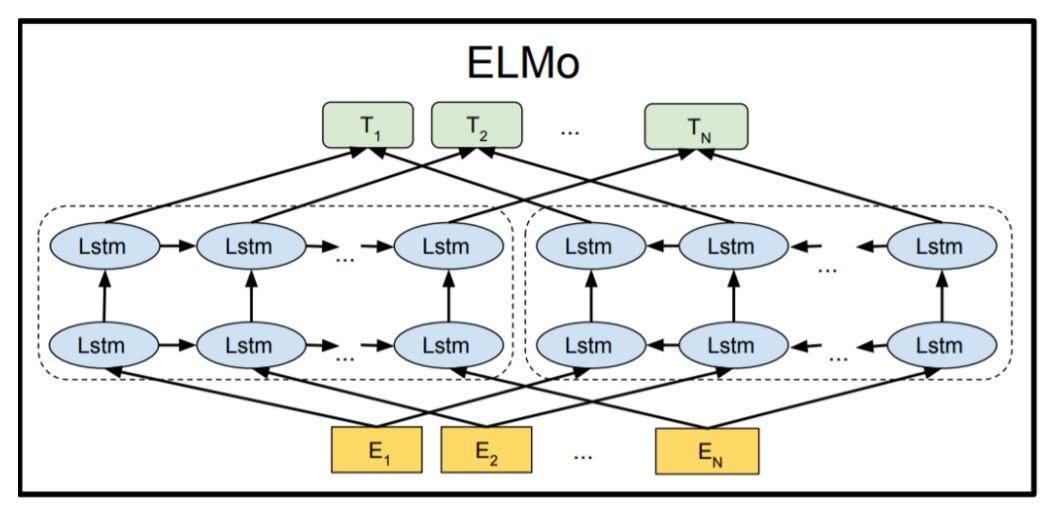
Fig.14 - Architecture of the ELMo language model

The main part of ELMo, the two bidirectional LSTMs are more or less straight forward. A more interesting part is the embedding part (E1,E2,…,En). This will be explained in more detail in the upcoming sections.

3.7.3 ELMo embedding

In the paper "Character-Aware neural language models", they propose a language model that leverages subword informations through a character-level convolutional neural network (CNN), whose output is used as an input to a recurrent neural network language model (RNN-LM). If we study the architecture in figure 15 in more detail, we can see that the ELMo is quite similar to the character-aware neural language model approach from 2015. They changed the simple vanilla LSTM to a bidirectional LSTM model, but the embedding part is in both approaches the same.

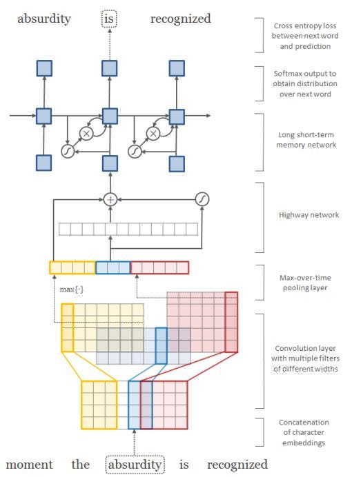
Fig.15 - Architecture of the word embedding as a preprocessing step for the ELMo model

The first layer performs a lookup of character embeddings (in the example above it is four dimensional) and stack them to the matrix C_k. On the matrix C_k are applied multiple filters (convolutions). In the example above, there are in total twelve filters - three filters with width of two (blue) four filters with width of three, and five filters with the width of four. On the resulting matrices of the filters is applied a max-over-time pooling operation, to obtain a fixed-dimensional representation of each word. This vector is used as input for the highway network. The output of the highway network will be used as input for the first bidirectional LSTM layer in the ELMo architecture.

3.7.4 Character-level convolutional neural network

Let assuming that C is the (one-hot encoded) vocabulary of characters. We can assume that the dimensionality will be 26 (every character in the alphabet). With this two informations we can build up the matrix for the character embeddings Q. The chracter-level representation of a word k with length l is given by the matrix C_k, where the j-th column in C_k corresponds to the character embedding for c_j in Q. In a next step several filters are applied on the matrix C_k. Finally they using a max-over-time pooling, to make sure, that each word have the same length as input of the highway network.

3.7.5 Highway network

The next step after the character-level CNN is the highway network. The authors of the paper refer to networks with this architecture as highway networks, since they allow unimpeded information flow across several layers of information highways. The main idea of the introduction of highway networks was, that many recent empirical breakthroughs in supervised machine learning have been achieved through the usage of deep neural networks. However, the training process of deep neural network is not as straight forward as simply adding additional layers to the architecture. Highway networks were a novel approach for the optimization of networks with a virtually arbitrary depth. The approach uses a learned gating mechanism, similar to the LSTM, or RNN gates, with this gating mechanism, the network can have paths along, which some informations can be processed through several layers without attentuation. This is a similar approach as the residual skip connections, which will be shortly explain in a later stage of this blog.

This model uses as input the max-over-time pooled vector, at least in the ELMo approach, created from the character-level CNN. The authors of the paper showed, that it is also possible in principle to feed the output of the charactet-level CNN yk directly to the LSTM layer. But the authors observed, that feed yk through a highway network before the LSTM will lead to some improvements of the accuracy. Highway networks in general can also be used in many other machine learning and deep learning problems. The word embedding in the ELMo approach is just one specific application of the highway network approach.

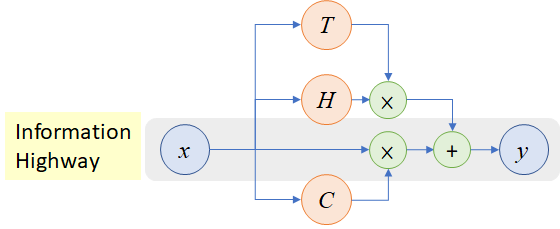
Fig.16 - Overview of a highway layer

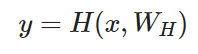
A plain feedforward neural network consists mainly of L layers and each layer applies a non-linear transformation H, where H is normally a affine transformation function, followed by a non-linear activation function (sigmoid, ReLU, etc.).

For the highway network, the authors introduced two additional non-linear transformations, T(x,W_T) and C(x,W_C). This yields to the following formula.

A layer of the highway network does the following:

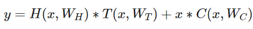
whereas C = 1-T and therefore:

where H is the non-linearity from a plain feedforward layer and T and C are the two additional introduced non-linearities. T is called the transform gate and (1−T) or C is called the carry gate. Similar to the memory cell in LSTM networks, highway layers allow for training of deep networks by adaptively carrying some dimensions of the input directly to the output. A more detailed explanation of the highway network can be found in the paper "Highway Networks"

3.7.6 ELMo summary

Sum up the most important features

• Contextual: The representation for each word depends on the entire context in which it is used.
• Deep: The word representations combine all layers of a deep pre-trained neural network.
• Character based: ELMo representations are purely character based, allowing the network to use morphological clues to form robust representations for out-of-vocabulary tokens unseen in training.

4. Sequence to sequence Models

The approach of squence to sequence models, or short seq2seq models, was introduced in 2014 by Google. The aim is to map a input vector with a fixed length to a output vector also with a fixed length, but maybe the length of the input and output is different. The model consists basically of a encoder part (one RNN or LSTM layer) and of a decoder part (another RNN or LSTM layer).

4.1 Encoder - Decoder principle

An encoder processes the input sequence and compresses the information into a context vector h_t of a fixed length. The decoder is initialized with the context vector h_t to emit the transformed output. The encoder consists of embedding layer followed by a RNN layer or a LSTM layer. The power of this model lies in the fact that it can map seqeunces of different lengths (input and output vector).

A basic Seq2Seq model can work quite well for short text sequences, but it has difficulties with long sequences, because the context vector has a fixed length and has to encode a lot of infomation. One possible solution to overcome the problem of long sequences, is to plug in the attention mechanism.

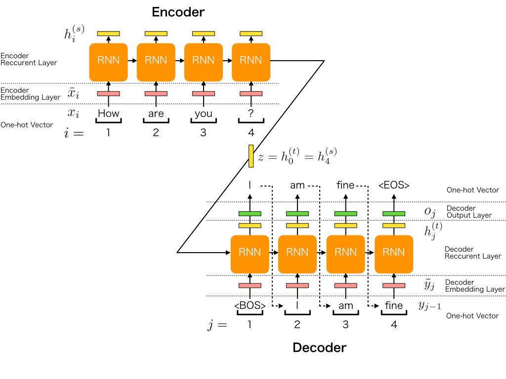
Fig.17 - Sequence to sequence architecture

5. Attention mechanism

In the previous architecture (sequence-to-sequence models), the encoder compressed the whole source sentence into a single vector, the so called context vector h_t. This can be very hard - the number of possible meanings of source is infinite. When the encoder is forced to put all information into a single vector, it is likely to forget something. Not only it is hard for the encoder to put all information into a single vector - this is also hard for the decoder to extract all important information from the context vector h_t. The decoder sees only one representation of source. However, at each generation step, different parts of source can be more useful than others. But in the current setting, the decoder has to extract relevant information from the same fixed representation.

An attention mechanism is a part of a neural network. At each decoder step, it decides which source parts are important for the decoder. In this setting, the encoder does not have to compress the whole source into a single vector - it gives representations for all source tokens (for example, all RNN states instead of the last one).

5.1 Mathematical background of attention mechanism

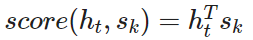
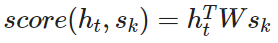
There are mainly three different ways to compute attention scores:

• dot-product - the simplest method:

• bilinear function (aka "Luong attention") more details could be find in the original paper

• multi-layer perceptron (aka "Bahdanau attention") more details could be fint in the original paper

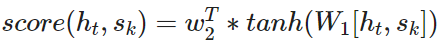
5.1.1 Bahdanau model

The encoder of the bahdanau model has two RNNs layers, one forward and one backward (bidirectional) layer, which reads input in the both directions. For each token, states of the two RNNs are concatenated. To get an attention score, apply a multi-layer perceptron (MLP) to an encoder state and a decoder state. Attention is used between decoder steps: state h(t−1)_ is used to compute attention and its output, and both h(t−1)_ and its outputs are passed to the decoder at step t.

5.1.2 Luong model

The encoder of the luong model uses only one unidirectional RNN layer. The attention mechanism is applied same as in the bahdanau model, after the RNN decoder step t before making a prediction. State h_t used to compute attention and its output. The luong model uses a simpler scoring function (bilinear) than the bahdanau model.

5.2 Self-attention mechanism

The self-attention mechanism was introduced in the paper "Attention is all you need". This approach is similar to the basic attention mechanism which was shown before. Self-attention is one of the key components of the transformer architecture, which we will explain in section 6 in more detail. The difference between attention and self-attention is that self-attention operates between representations of the same nature: e.g., all encoder states in some layer. Self-attention is the part of the model where tokens interact with each other. Each token "looks" at other tokens in the sentence with an attention mechanism, gathers context, and updates the previous representation of "self".

Formally, this intuition of self-attention is implemented with a query-key-value attention. Each input token of a self-attention layer receives three representations (matrices) corresponding to the roles it can play:

• query - asking for information
• key - saying that it has some information
• value - giving the information

The self-attention function can be described as mapping a query (W_Q) and a set of key-value (W_K, W_V) pairs to an output. The input consists of a query vector and key-value vectors (dimension of values: d_v, dimension of keys: d_k). Based on these three vectors the self-attention layers calculates the three matrices W_Q, W_K and W_V. With these three matrices we can calulate the attention weigths (the output matrix of the attention layer).

Formula to calculate the self-attention output:

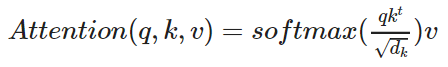
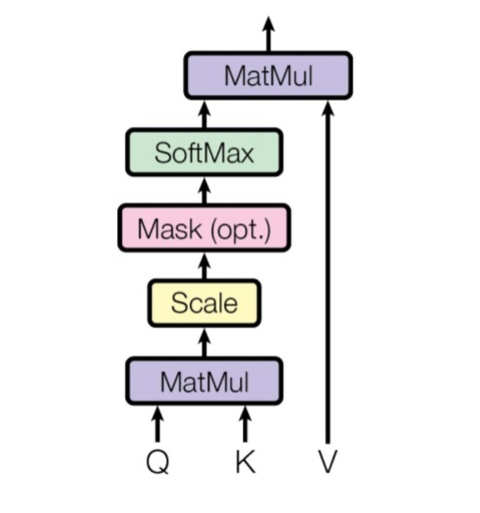
Fig.18 - Overview of the self-attention mechanism

5.3 Multi-head attention mechanism

The multi-head attention mechanism is an extension of the self-attention mechanism and is also implemented in the transformer architecture. The main idea of the authors of the paper was, instead performing a single attention function with d_model-dimensional keys, values and queries, it would be beneficial to linearly project the queries, keys and values h times with different, learned linear projections (the W_K, W_Q and W_V matrices).

where:

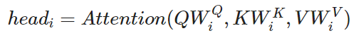
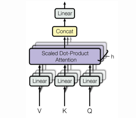
Fig.19 - Overview of the multi-head attention mechanism

6. Transformers

Transformers are introduced in 2017, in the paper "Attention is all you need". It is based solely on attention mechanism: i.e., without recurrence (RNN’s) or convolutions (CNN’s). On top of higher translation quality, the model is faster to train by up to an order of magnitude. Currently, Transformers (with variations) are de-facto standard models not only in sequence to sequence tasks but also for language modeling and in pretraining settings.

Transformer introduced a new modeling paradigm. In contrast to previous models where processing within encoder and decoder was done with recurrence or convolutions, transformer operates using only attention. The original transformer model uses the outputs of the decoder as input for the next prediction step, as shown in figure 20. We will see in the next sections, that some newer versions of the transformer only uses the encoder part or only the decoder part.

The transformer architecture is a stackwise architecture, it is simply possible and also useful to stack several encoder- and decoder layer together. The number of stacks could be a hyperparameter, which should be tuned during training, as well the number of attention head and the dimensions of the Q,K and V matrices of the self-attention layer.

6.1 Transformer architecture

Fig.20 - Overview of the transformer model

6.1.1 Positional encoding

Similiar to the previous shown NLP models, the transformer approach also uses learned embeddings to convert the input tokens and output tokens to vectors of dimension d_model. It is possible to use the Word2Vec embedding, to convert the input words to a continuous vector with a predefined dimension.

The transfomer model contains no recurrent (RNN’s or LSTM’s) an no convolutions, in order to make use of the order of a sequence, it is necessary to insert informations about the relative and absolute position of the input tokens of the model. The authors introduced as an additional embedding step the so called positional embedding, which is applied after the classical word embedding.

Mathematical formulation of the positional encoding approach:

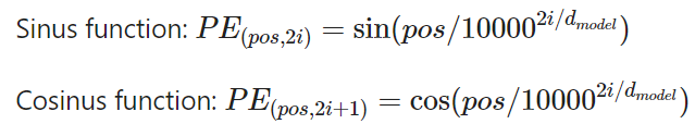
The final positional encoding which is then used as input of the transformer is simple a sum of the embedding vector and the positional vector. For example if we consider the word "black", the positional vector is calculated as follow:

pc(black)=embedding(black)+pe(black), therefore it is necessary that the embedding vector and the positional vector have the same dimensions, mostly 512 dimensions.

6.1.2 Feed forward blocks

Additionally to the attention layers, each stack of the encoder and decoder contains one feed forward network. This layer consists of two linear layers with ReLU non-linearity in between. After looking at other tokens via an attention mechanism, a model uses an feed forward network block to process this new information.

Mathematical formulation of the feed forward layer:

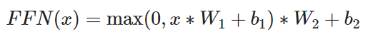
A feed forward layer could be build out of convolutional layer with kernelsize = 1. The network used in the paper "Attention is all you need" has a input and output dimensionality of d_model = 512 and the inner layer has a dimensionality of d_ff = 2048.

6.1.3 Residual connections

Residual connections are very simple (add a block’s input to its output), but at the same time are very useful. They ease the gradient flow through a network and allow stacking a lot of layers. In traditional, basic neural network architectures each output of a layer is feed into the next layer. The authors of the paper "Deep Residual Learning for Image Recognition" showed that deeper network not always ends up with smaller training and test errors. Therefore the residual connections can be very useful for deep networks, for skipping some layers that do not help to improve the model accuracy.

In the transformer, residual connections are used after each multi-head attention and feed forward network block.

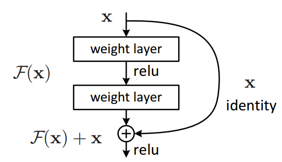
Fig.21 - Residual block

6.1.4 Layer normalization

The layer normalization, which is applied after the multi-head attention layer contains a add and normalization function. The add function is used to sum up the output of the multi-head attention and the residual connection, which comes directly from the input of the attention layer. The layer can be described as follows:

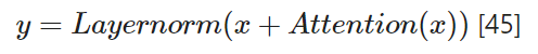
Many different methods exists for the layer normalization, but we will not go in detail in this blog.

6.2 GPT language model

The GPT-1 GPT-2, or GPT-3 are highly advanced models for several NLP taks. These models were introduced by OpenAI. The licence of the actual GPT-3 model was sold to Microsoft and is no longer accessible for the community. OpenAI showed with the GPT-2 and 3 in a very impressive way how fast the reasearch and developement is still going on. The transformers went from training from scratch over fine tuning on a specific task to finally zero shot, or few shots models in less than three years. The newest zero-shot / few-shot GPT-3 model requires no fine tuning for each downstream task and showed quite impressive results in some NLP taks, more details about the GPT-3 paper.

OpenAI was reaching the goal of using a GPT model on a downstream task without fine tuning, with the following four steps:

• Fine tuning: A transformer was trained on a large corpus of data (this could be done in a unsupervised way). Afterwards the trained model was fine tuned specifically on a downstream task.
• Few shot: This step represents a hugh step forward. As startingpoint there is still a pretrained model. When the model needs to make inferences, it is presented with some examples of the task to perform as conditioning. Conditioning replaces weight updating.
• One shot: This step takes the process yet further. The pretrained GPT model is presented with only one demonstration of the downstream taks. There will be no weight updating
• Zero shot: The pretrained GPT model is presented with NO example of the downstream task. Therefore the GPT model must be able to generalize very good on mostly all NLP problems.

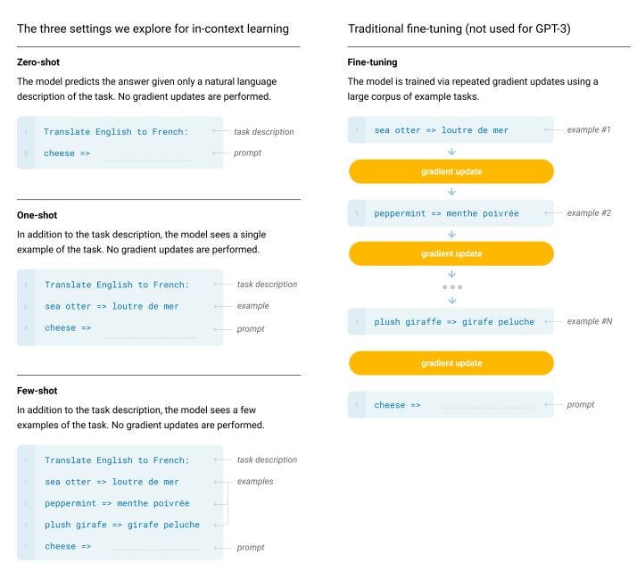
Fig.22 - Symbolic example of the different learning approaches in the GPT models

The main goal of OpenAI is to generalize the concept of understanding language to any downstream taks. Therefore the training is highly intensive and requires a hugh amount of data, because the GPT model rapidly envolved from 117M parameters (GPT-2 small) to 345M parameters (GPT-2 medium) to 762M parameters (GPT-2 large) and 1,542M parameters (GPT-2 extra large).. The newst GPT-3 model has incredible 1.5 billion parameters.

All GPT model uses only the decoder part of the original transformer architecture, shown in figure 23 below. In comparison to the BERT model, GPT do not use a bidirectional approach. More about a step-by-step implementation of a GPT model could be found in the book "Transformers for natural language processing" written by Daniel Rothman.

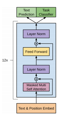
Fig.23 - Overview of the GPT model archtiecture

6.3 BERT (Bidirectional encoder representations from transformers)

The BERT model, a new language representation model from Google AI, uses pre-training and fine-tuning to create state-of-the-art models for a wide range of tasks. These tasks include question answering systems, sentiment analysis, and language inference. BERT uses a multi-layer bidirectional transformer encoder. The self-attention layer performs self-attention in both directions. Google has released two variants of the model:

• BERT Base: Number of transformers layers = 12, total parameters = 110M
• BERT Large: Number of transformers layers = 24, total parameters = 340M

The BERT approach uses a semi-supervised training approach. The model was pretrained on a large text corpus without any labels (unsupervised learning). Google AI used the the WordPiece word embedding, with 30'000 tokens vocabulary. The BERT model was trained on the BookCorpus with 800 million words and the English wikipedia with 2500 million words. The pretraining contains two different NLP taks. First, "masked language modeling (MLM)" and "next senctence prediction (NSP)".

Masked language modeling

Masked language modeling does not require training a model with a sequence of visible words followed by a masked sequence to predict. Here a short example from the book "Transformers for natural language processing":

• "The cat sat on it because it was a nice rug"

The decoder would mask the attention sequence after the model reached the word "it":

• "The cat sat on it masked sequence"

But the BERT encoder masks a random token to make a prediction:

• "The cat sat on it MASK it was a nice rug"

The multi-head attention sub-layer can now see the whole sequence, run the self-attention process, and predict the masked token.

next sentence prediction

In this approach the input contains always two sentences. Therefore two new tokens were added:

• CLS this is a binary classification token, added to the beginning of the first sentence to predict, if the second sentence follows the first one. A positive sample is a pair of two consecutive senctences taken from a dataset. A negative sample is created using sentence from different documents.
• SEP is a separation token that signals the end of a sequence.

The aim is now to learn, if the two sentence are two consecutive sequences from one document or not.

6.3.1 BERT finetuning

The usage of a BERT model for a specific downstream taks is relatively straightforward. There are many different versions of pretrained models available. A very good pasge is https://huggingface.co/models. After loading a pretrained version of the BERT model, it is necessary to fine tune the parameters of the model. It is also necessary to add one addtitional output layer and a input layer if needed. For a Q & A Bot we have three inputs, the context a answer an a corresponding answer which should be find in the context. Figure 24 shows symbolic the idea behind the pretraining and fine tuning process.

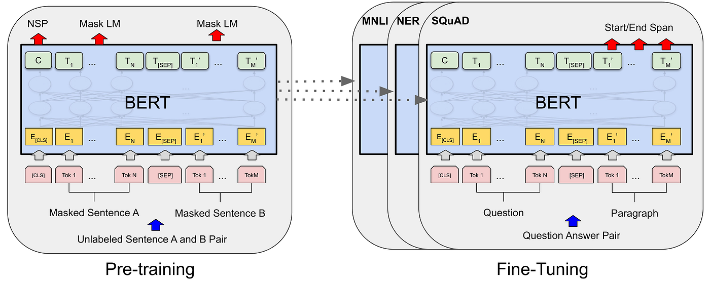
Fig.24 - Two steps of using a BERT Transformer

6.3.2 Comparison of the different models

Figure 25 below, shows the main differences in pre-training model architectures. The BERT model uses a bidirectional Transformer. The GPT model from OpenAI uses a simple left-to-right transformer. The ELMo model does not use the transformer approach, as we have seen earlier in this blog. Therefore the BERT and GPT model performs better than previous approaches including ELMo. Until today, various versions, with some small changes or adaptions have been introduced, but all of these models still using the transformer model at the core.

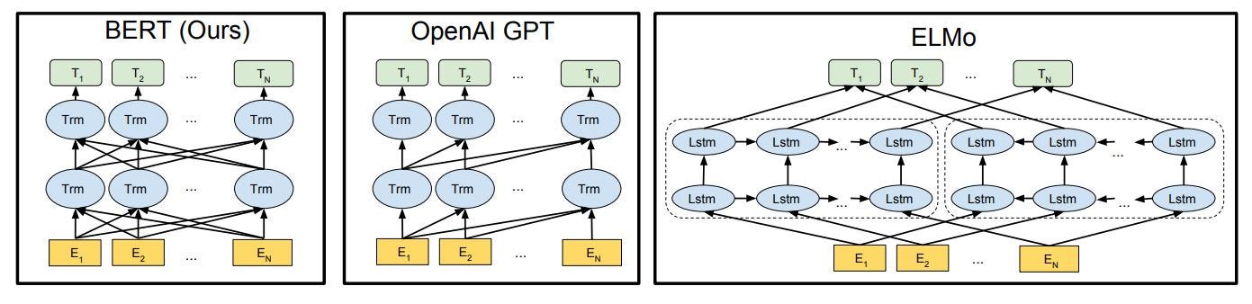
Fig.25 - Two steps of using a BERT Transformer

7. Practical Example

Check out the following Github repository, this blog can also be found there as a HTML file, with additional practial python examples.

https://github.com/robinvetsch/Transformer_SQUAD.

NLP - From Word Embedding to Transformers | by Robin | Medium

Others

Mamba

Shortcomings of Transformers

• Transformer models are widely used for language modeling tasks.
• They suffer from a quadratic attention mechanism, which makes them slow for long sequences.
• The slowness of Transformers for long sequences limits their usefulness.

How Mamba is solving these problems

• Mamba is a new model that uses an SSM architecture for linear-time scaling.
• It is based on S4, a state space model, which can be discretized for use with text data.
• Mamba can be used in two modes: RNN mode and CNN mode. RNN mode is better for inference while CNN mode is better for training.
• Mamba introduces selectivity to the model by making the model parameters dependent on the input.

Mamba is a linear-time language model that outperforms Transformers on various tasks. It achieves this speedup by using a combination of techniques including an SSM architecture and recurrent updates. Overall, the post explains how Mamba solves mostly long sequence limitations especially Transformer being computationally expensive to understand and model long sequences of user interactions.

Mamba: The Easy Way

Mamba Explained